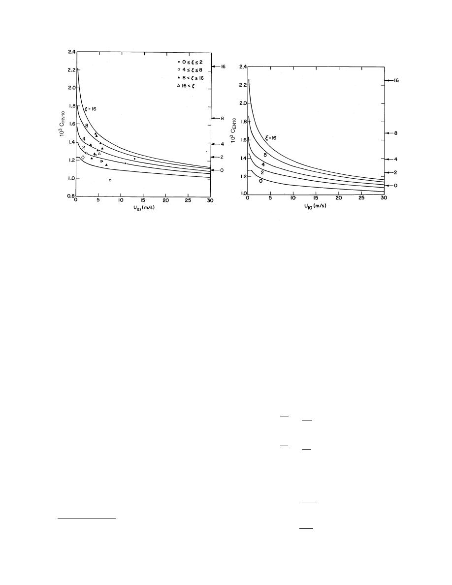
b. CEN10.
a. CHN10. The data points are from measurements by
Kondo and Yamazawa (1986).
Figure 20. Model predictions (from Andreas 1987) of CHN10 and CEN10 over snow-covered surfaces as a function of
the surface roughness parameter ξ (in cm) and the 10-m wind speed, U10. The arrows on the right show CDN10 for the
indicated ξ value.
tion for these observations and thereby provided meteor-
1 m), I had to obtain their raw data* to compute the
ology and oceanography with the first rigorous planetary
points plotted in Figure 20a. In addition, because they
had not measured ξ, I inferred the ξ values associated
boundary layer model. Though the spiral in the wind
vector that Ekman's model predicts is rarely seen, his
with the CHN10 values in Figure 20a by using eq 111 to
estimate ξ from their measured drag coefficients.
model is still a basis for current ABL modeling. Hence,
I will describe it in some detail here.
Although there are some discrepancies between the
Start with eq 16, which are equations for the mean
model predictions and the data in Figure 20a, the com-
horizontal wind vector. Assuming steady-state simpli-
parison is quite encouraging. The data support the model
fies these, but the turbulence terms still make analytic
prediction that CHN10 increases with increasing CDN10
solution difficult. We, thus, need a closure assumption.
at a given wind speed and that CHN10 decreases with
The Ekman solution is to assume that the turbulent trans-
increasing wind speed. Unfortunately, no high quality
port can be modeled as a turbulent diffusion process
measurements are yet available for testing the model's
with a constant turbulent diffusivity K. That is, the sur-
prediction for CEN10, though several have accepted its
face stresses in the x and y directions, τx and τy, are
predictions for both CHN10 and CEN10 (Morris 1989,
modeled as
Munro 1989, Launiainen and Vihma 1990).
U
τx / ρ = -uw = K
(114a)
THE EKMAN LAYER
z
Polar meteorology has, of course, relied on the dis-
V
coveries of meteorologists working at lower latitudes.
τy / ρ = -vw = K
.
(114b)
z
But, in turn, meteorologists and oceanographers every-
where owe a debt to a polar scientist, Fridtjof Nansen.
With these and the assumption of steady-state, eq 16
During the drift of the Fram across the Arctic Ocean in
yield (e.g., Stull 1988, p. 210 f.; Garratt 1992, p. 42)
the mid-1890s (Nansen 1897), Nansen noticed that his
ship and the sea ice generally drifted to the right of the
2
U
- f (V - Vg ) = K
wind. Ekman (1905) developed a mathematical explana-
(115a)
z2
2
V
f (U - Ug ) = K
* Personal communication with J. Kondo, Professor of Meteorol-
(115b)
z2
ogy, Geophysical Institute, Tohoku University, Sendai, Japan, 1986.
23


 Previous Page
