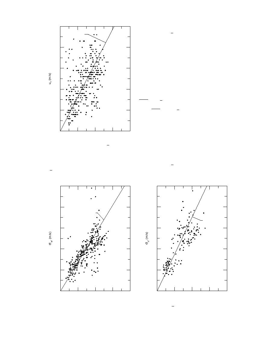
and
0.5
σ′ = 0.35 u2m .
(74)
u = 0.079 u 2m
u
*
The value of 0.113 is slightly lower than that in
0.4
eq 66, but the value of 0.35 is identical to the one
given in eq 67. Figure 12 shows the variation of
σ u′ and u* for the same measurement period and
can be expressed by
0.3
σ u′ = 3.68 u* ,
(75)
which is more or less the same as the relation
0.2
shown in eq 68.
Figure 13 shows the variation of covariance
w′ T ′ with u2m . It can be represented by
w′ T ′ = 0.014 u2m .
0.1
(76)
The constant 0.014 is only one third of the value
given in eq 71. Neglecting the effect of variation
of ρ and cp with temperature and atmospheric pres-
0
0
2
4
6
8
sure, the sensible heat flux is only one third of the
u 2m (m /s)
_
value during the late spring to early summer.
Figure 10. Variation of u* with u2m based on
Though the data points in all these figures are
data taken in late fall, winter, and early spring.
scattered to a great extent, the least-squares cor-
relation coefficients of all these linear relations,
i.e., eq 7176 are greater than 0.8313 (as high as 0.9716 for σ u′ vs. u2m ). It indirectly indicates that
u2m is the predominant factor in correlating this type of data.
2.0
1.0
1.6
0.8
σw' = 0.133 u 2m
σu' = 0.35 u2m
1.2
0.6
0.8
0.4
0.4
0.2
a.
b.
0
0
0
2
4
6
8
0
2
4
6
8
u
_ 2m (m /s)
u
_ 2m (m /s)
Figure 11. Standard deviations σ w′ (a) and σu′ (b) as a function of u2m based on data taken in late
fall, winter, and early spring.
28


 Previous Page
