20
15
10
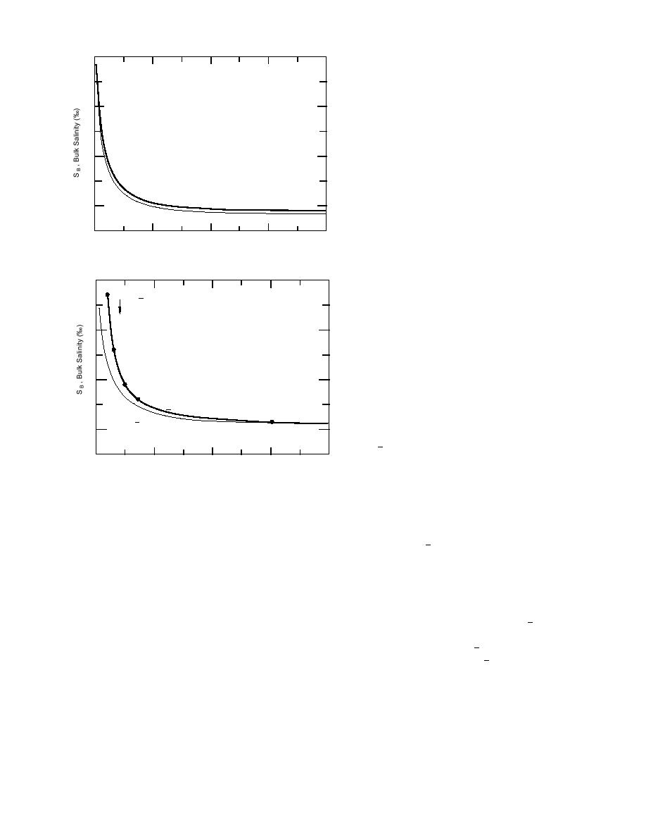
S w = 34 ‰ (Amundsen and Bellingshausen Seas)
5
S w = 31.5 ‰ (Beaufort Sea)
Figure 12. Sea-ice bulk salinity vs. floe thickness
as calculated with Ryvlin's equation for 31.5 and
0
50
100
150
200
34‰ seawater.
TF , Floe Thickness (cm)
20
0.220 = a
15
0.320
10
0.375
0.400
a = Varied
0.450
Figure 13. Ryvlin's equation for calculating sea-
a = 0.5
ice bulk salinity vs. floe thickness where param-
5
eter a is constant (lower curve) and varied (up-
per curve) to match the regression curve through
0
50
100
150
200
the Beaufort Sea ice data in Figure 11.
T F , Floe Thickness (cm)
Arctic (Fig. 11) and Antarctic (Fig. 14) are not
SBF = 5.41‰ at TF = 200 and dividing this salinity
sufficient to fully define the SB vs. TF trends or
by Sw = 34‰ gives an SR of 0.159. Using this
that the effect of the seawater salinity differ-
value in eq 1 gives the lower curve in Figure 15.
Varying coefficient a at the TF increments shown
ence on SB is masked by the scatter in the data
and/or ice structure differences. Perhaps as im-
in Figure 15 causes the Ryvlin equation to give SB
portant is the regression curve selected to repre-
vs. TF values that match the regression curve
sent the data. Statistically, two regression curves
through the Antarctic data (Fig. 14). Both the modi-
may fit the data with nearly the same correlation
fied Ryvlin and regression curves are represented
coefficient r2 value, but they give different SB val-
by the upper curve in Figure 15.
ues at 200 cm. In any event, since the regression
The fact that growth rate coefficient a needs
curves (Fig. 11 and 14) lie well within each other 's
to vary with TF is not surprising. Ryvlin indicated
standard deviation, there is no statistically sig-
as much in his description of a in eq 1. A further
nificant difference between them. Given this rea-
indication of the need to vary a can be seen in
soning, it would seem that the Arctic and Antarc-
Figure 8. Here the time to grow successive incre-
tic sea ice SB vs. TF data can be combined.
ments of ice is shown to increase with thickness.
Also shown in Figure 14 is the curve derived
In short, the heat flux through growing sea ice
from unmodified eq 1 (Fig. 12). As with the Beau-
decreases exponentially with thickness and like-
fort Sea data, the curve does not fit the data.
wise reduces the rate of ice growth (Makshtas
Taking the regression curve (Fig. 14) value for
1984, Maykut 1986) and brine entrapment. The
8


 Previous Page
