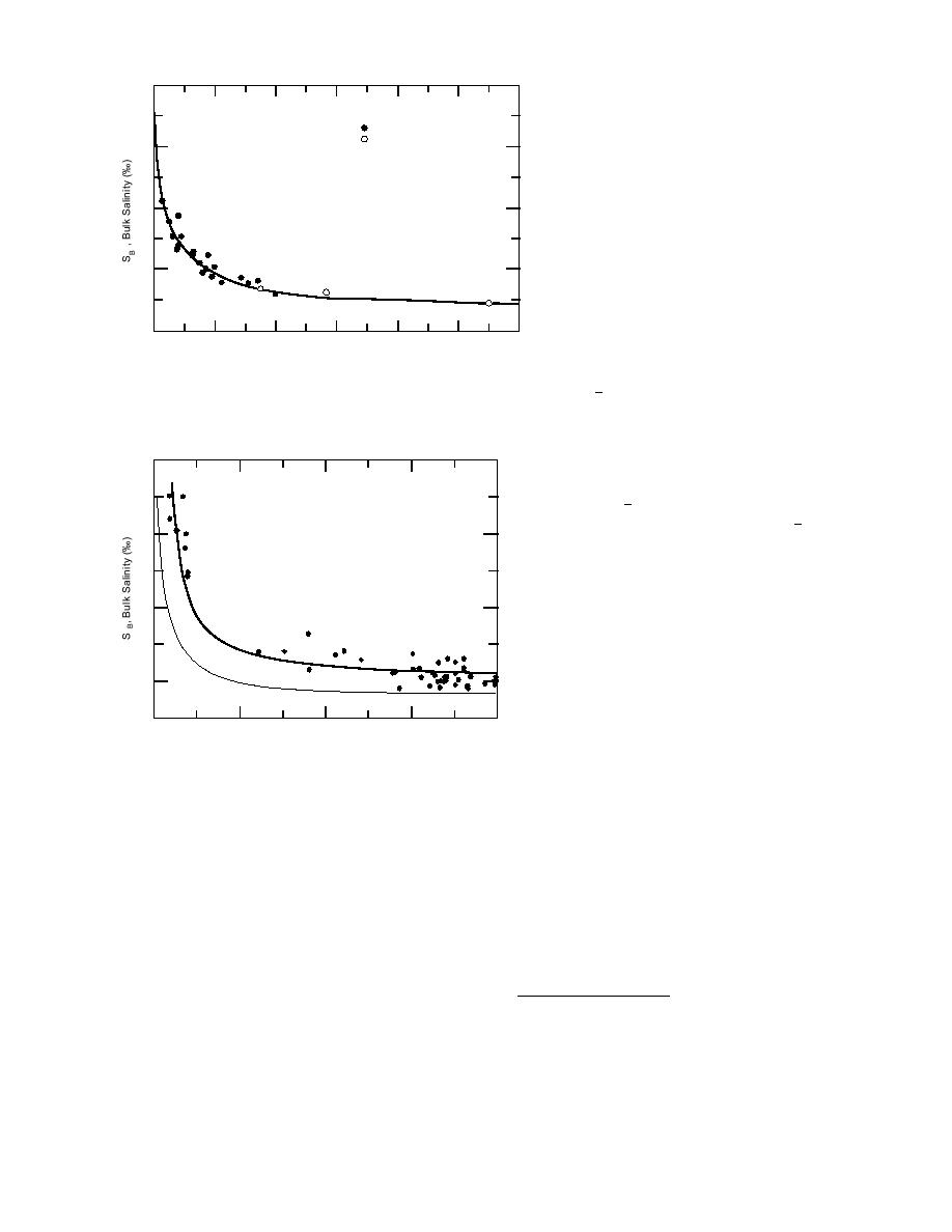
eq 1 does not fit the data. This is surpris-
40
ing, given the good agreement shown in
Figure 10.
Weeks and Anderson
Ryvlin
At 200 cm the regression curve in Fig-
30
ure 11 gives a value of 5.50‰ for SB. Divid-
ing this salinity by Sw = 31.5‰ gives a
value for SR of 0.175, not 0.13 as Ryvlin
20
determined from his data analysis. Using
this new SR value along with his suggested
growth rate coefficient of 0.5 in eq 1 brings
10
the Ryvlin curve into good agreement with
the regression curve between TF = 125 and
200 cm. However, there is still a significant
difference between eq 1 and the regression
0
40
80
120
20
60
100
curve where TF is less than about 50 cm. To
T F , Floe Thickness (cm)
bring the two curves into agreement, coef-
Figure 10. Comparison of Ryvlin's empirical equation for esti- ficient a has to vary with T . This is shown
F
mating sea-ice bulk salinity vs. floe thickness, with field data in Figure 13, where the lower curve repre-
(after Ryvlin 1974).
sents eq 1 with only SR changed from 0.13
to 0.175 and the upper curve represents
both the regression line through the data
20
in Figure 11 and eq 1 with SR = 0.175 and
2
S B = (2.242 + 20.556/TF)
coefficient a varied as shown.
2 = 0.840
r
To verify the need to vary SR and a in eq
S D = 1.45
1, I analyzed the SB vs. TF data collected by
15
Jeffries (1994) in the Amundsen and
Bellingshausen Seas, Antarctica, in late
winter. Unlike the predominantly congela-
10
tion sea-ice data from the Arctic (Beaufort
Sea) the Antarctic sea-ice data are from ice
sheets having a predominantly frazil, large
interlaced platelet and infiltrated snow ice
5
structure. Core data on ice up to 200 cm
thick with a mean temperature below 3C
S w = 31.5 ‰ (Beaufort Sea)
were selected. The latter ensured that the
0
50
100
150
200
T F, Floe Thickness (cm)
ice was "cold" and not melting. Their data
from 74 ice cores are shown in Figure 14.
Figure 11. Beaufort Sea first-year ice bulk salinity vs. floe thick-
T h e re p r e s e n t a t i v e re g r e s s i o n c u r v e
ness. The lower curve represents the results of Ryvlin's equa-
through the data is of the same form as the
tion for 31.5‰ seawater.
one through the Beaufort Sea ice data in
Figure 11. It is important to note that the re-
linity difference caused an 8% difference in the
gression curve at TF = 200 cm gives SB = 5.41
bulk sea-ice salinity.
The regression curve through the Beaufort Sea
vs. 5.50‰ for the Beaufort Sea data. Given the
SB vs. TF data (Fig. 11) is, for all intents and pur-
fact that the Antarctic seawater salinity is 34‰*
poses, horizontal after an ice thickness of about
vs. 31.5‰ for the southern Beaufort Sea, one
150 cm. Therefore, SBF may be determined from
would expect these SB values to be reversed for
the regression curve at any TF after 150 cm with
reasons previously discussed. This unexpected
minor effect on the results of eq 1. For consis-
result suggests that the sea-ice data for the
tency, SBF at TF = 200 cm is used in this report.
Running below the regression line, and most
* M. Jeffries (1995), Geophysical Institute, Univer-
of the data, in Figure 11 is the curve derived using
sity of Alaska, Fairbanks, and S. Jacobs (1995),
eq 1 and an Sw of 31.5‰ (Fig. 12). Even though
Lamont-Doherty Geological Observatory of Colum-
the number of data points is limited (and non-
bia University, Palisades, New York, personal com-
existent for a TF of 25 to 50 cm) it is apparent that
munications.
7


 Previous Page
