

In principle, the NSRSIM01 (Northern Sea Route
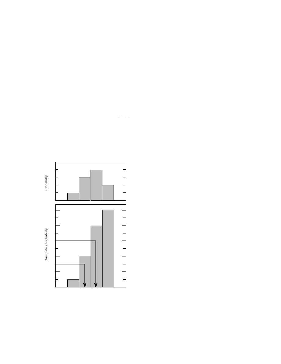
category, and for R = 0.60, thickness is in the 120 to
Simulator--Version 01) model works in this man-
240 cm category. Using this same logic, randomly
ner. The likelihood that a particular variable will
selected values of 0.10 and 0.90 would fall in the
assume a given value is described by a probability
ice-free and >240 cm categories, respectively.
density function (PDF) that is based in most cases
Inasmuch as R is drawn from a uniform distri-
on observational data acquired over long time pe-
bution, all values within the range that R can as-
riods. A variable is initialized by making a ran-
sume are equally likely to be selected. On average,
dom drawing, weighted by the PDF, from the
10% of the time R will fall between 0.0 and 0.1,
range of possible values the variable can assume.
meaning that the ice-free category, which has a
Take, for example, a hypothetical case in which ice
probability of occurrence of 0.1, will be chosen once
thickness observations at some point along the NSR
in every ten selections. The 0 to 120 cm category,
produce the PDF shown in Figure 2. MC sampling
with a probability of 0.3, will be selected three
of this distribution as implemented in the
times in ten, or when R is between 0.1 and 0.4.
NSRSIM01 algorithm involves first converting this
Over the long term, an ice thickness distribution
raw PDF to a cumulative probability distribution
produced through many iterations of this algo-
(Fig. 2), generating a random number R drawn
rithm would replicate the PDF in Figure 2. Thus,
from a uniform distribution such that 0.0 < R < 1.0,
to the extent that raw PDFs reflect environmental
and then selecting an ice thickness value on the
parameters accurately, the MC method simulates
basis of the value of R taken with respect to the
the frequency with which real-world conditions
occur.
cumulative probability distribution. Figure 2 shows
Our transit model uses the MC technique for
ice thickness selections based on two values of R:
calculating an average time and cost for shipping
for R = 0.30, ice thickness is in the 0 to 120 cm
between Murmansk, Russia, and the Bering Strait,
using the NSR. We selected the MC method as a
practical approach for addressing the many ran-
0.5
dom parameters that affect the cost of shipping.
A
Instead of relying on fixed input parameters, the
0.4
MC technique makes full use of the probability
0.3
density functions of input variables to calculate a
probable distribution of transit times and costs. In
0.2
this case, many of the environmental (atmospheric,
0.1
ice, and sea) conditions along the route are suffi-
0
ciently known at various times of the year to yield
distributions of their likelihood of occurrence. The
B
1.0
environmental conditions that are encountered on
a voyage affect the time needed for transit, which
in turn affects the cost of transit. For example, we
0.8
have sufficient data to say that near Cape Zhelaniya
(the northern tip of Novaya Zemlya) in August,
R = 0.6
the wind direction and wind speed have ranges of
0.6
known probabilities (see Table 2). When the ship
reaches that location, the model randomly selects
a weighted wind direction from the table (column
0.4
R = 0.3
2). Once the direction is set, the model then ran-
domly selects a weighted wind speed associated
with that direction (e.g., from row 3 for a 90135
0.2
wind direction).
For some conditions, such as fog, snowstorm,
0
Ice
0 to
120 to > 240
and icing, we have the probabilities of existence
Free
120
240
but not the additional knowledge of their magni-
Ice Thickness (cm)
tudes. So, for example, if there is a 20% historical
probability of fog occurring, then the random se-
Figure 2. Selection of ice thickness values
from a hypothetical probability density func-
lection for fog is weighted 80% in favor of clear
weather.
tion (PDF) using Monte Carlo methods.
7

 Previous Page
