Tension (kPa)
0
40
20
1
1
10
10
Taxiway A Subbase
γ d = 2.16 Mg/m 3
0
10
G s = 2.79
2
10
Calculated
1
Extraction
10
3
10
102
4
10
3
10
5
10
104
Sample 1171
5
6
10
10
0
100
200
300
400
500
80
85
90
95
100
Tension (cm water)
Degree of Saturation (%)
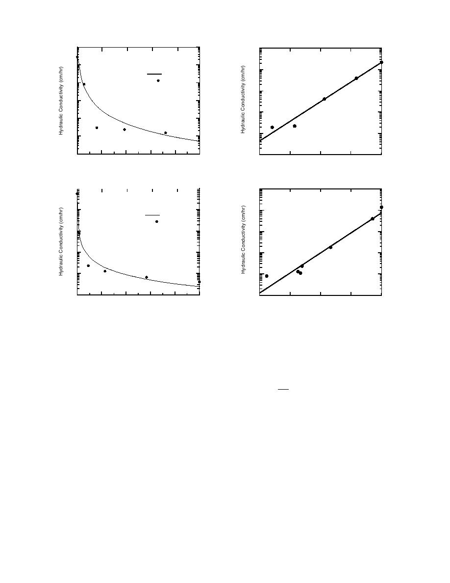
a. Subgrade sample 1171 (563)
g. Taxiway A subbase.
0
40
20
1
1
10
10
Dense-graded Stone
γ d = 1.89 Mg/m 3
0
10
2
G s = 2.80
10
Calculated
1
Extraction
10
3
10
2
10
4
10
3
10
5
10
4
10
Sample 1206
6
105
10
0
100
200
300
400
500
80
85
90
95
100
Tension (cm water)
Degree of Saturation (%)
b. Subgrade sample 1206 (565).
h. Dense-graded stone.
Figure 8. Degree of saturation vs. hydraulic
Figure 7 (cont'd). Tension vs. hydraulic con-
conductivity curves. Solid line is an exponen-
ductivity curves. Solid line represents Gard-
tial regression fitted to both the extraction
ner's equation approximation of the extrac-
and absorption data, when available.
tion data.
The best fit lines shown in Figures 7 and 8 are
β
-T
those that are generated from eq 1 and 2. Other
wu = α
; T < 0C
(3)
T0
equations may fit data from some samples better,
but the Gardner's form equation is that currently
where wu = gravimetric unfrozen moisture content
employed in the mechanistic design procedure.
(%)
T = temperature (C)
Unfrozen moisture content
T0 = 1.0C
The variation of unfrozen moisture content with
α and β = constants
temperature was determined by testing each mate-
rial with a pulsed nuclear magnetic resonance tech-
nique (Tice et al. 1982). The cooling curve data
Table 8 presents the constants determined for
are presented in Appendix E and in Figure 9. The
each sample. The class 6 special stockpile material
figure also includes a curve of calculated values
was split into two fractions above and below the no.
used to represent the data in the mechanistic pro-
30 sieve. The calculated curve represents the equa-
cedure, produced with an equation in the form:
tion developed for the minus no. 30 sieve fraction.
16


 Previous Page
