Figure 21. Ice floe σc values calculated using eq 8 from his study compared with the data provided by Sanderson

Figure 18. Equation-8-determined ice floe σc strengths vs. bulk porosity and strain rate (a) and the boresight view from the above strain rate window (b)

Figure 24. Ice floe σc values vs. bulk brine volume and strain rate (a) and the boresight view of the above from the strain rate window (b)

CR96_11
Page Navigation
12

ε, Strain Rate (s 1 )

, Strain Rate (s 1 )

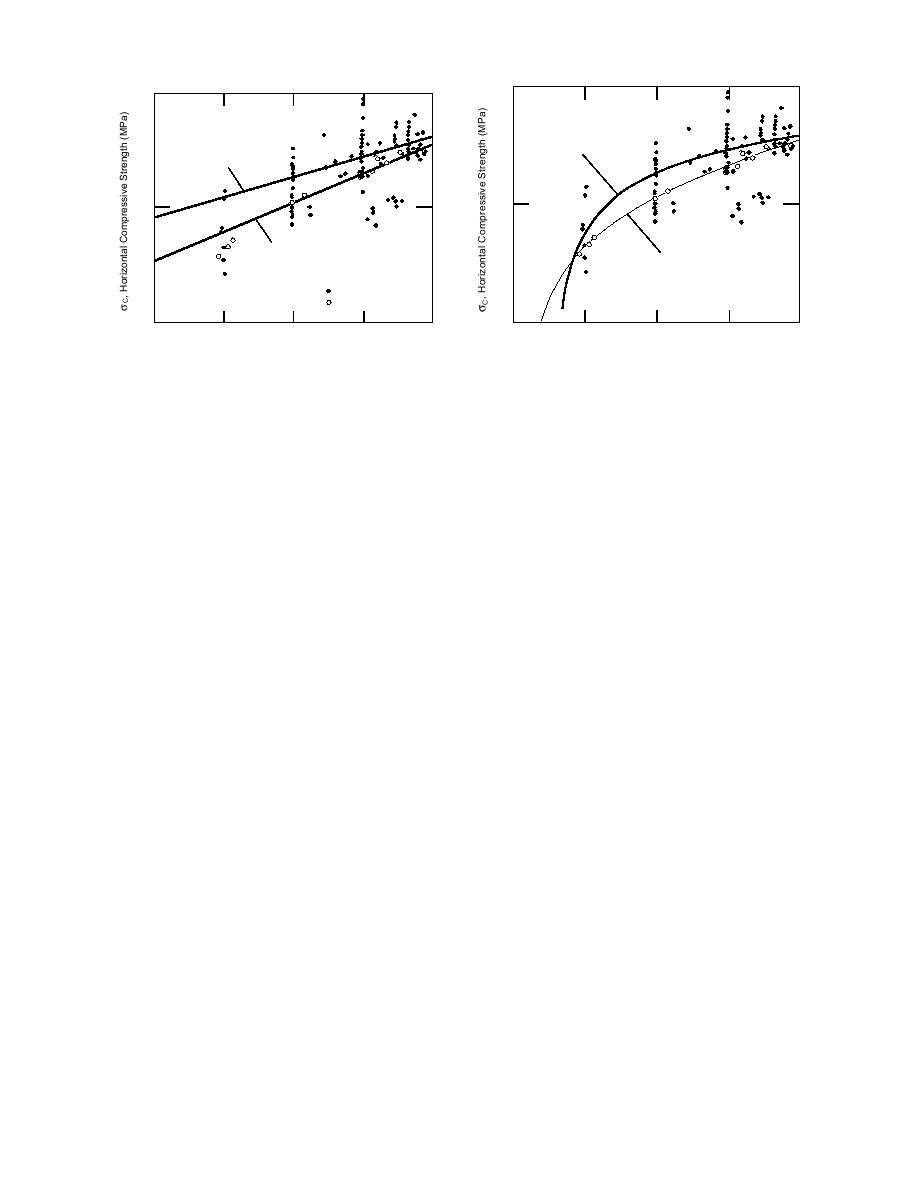
Figure 21. Ice floe σc values calculated using eq 8 from

Figure 20. Ice floe σc values calculated using eq 8 from

this study compared with the data provided by Sanderson

the study compared with the data provided by

(1988). The data were fitted with non-log-log power

Sanderson (1988). The data were fitted with a single-

equations.

term power equation.

presentation, no corrections have been made to

σc = 1970 ε0.32 φB0.95 .

(10)

the data to account for differences in test tech-

nique, ice porosity, grain size, or crystal orienta-

In the boresight view of the data from the strain

tion. This is not unusual since some of these pa-

rate window in Figure 22b, the "outlier" with

rameters were not measured or provided in the

the long offset tail at a strain rate of 7.9 107s1

original source material, as is the case for the

is very apparent. However, removing this data

Exxon data used in this report. For this reason

point and reanalyzing the remaining data gives

there is considerable scatter in the data. The up-

a new equation whose calculated σc values do

per regression curve shown in Figure 20 fits the

not vary by more than 0.04 MPa from those cal-

data from Sanderson; the lower curve represents

culated by eq 10.

the data generated from eq 8. The small amount

The form of the expression for the curved fail-

of data from this study coupled with the un-

ure surface shown in Figure 17 does not fit the

knowns mentioned above does not allow a defini-

new data set as well as the power type equation

tive statement to be made on the difference be-

in Figure 22. This may be seen by comparing the

tween the two lines. Clearly, the data from this

statistics listed in Figure 22 with those in Figure

study fit well within the scatter of the data from

23. The boresight view of the failure plane from

Sanderson. Both sets of data are statistically bet-

the strain rate window (Fig. 23b) also indicates no

ter represented by the nonlinear curves shown in

fit improvement for the outlier over the failure

Figure 21. Here again, the failure surface appears

surface shown in Figure 22b.

to be a non-power-law function of the strain rate.

Substituting the new νB data for the φB data

The Timco and Frederking (1990) study, which

and reanalyzing as before gives the results shown

resulted in the formulation of eq 6, is based on

in Figure 24. The expression for the failure surface

small-scale test results. How applicable this equa-

is now

tion is to full-scale ice force assessments can be

σc = 523.24 ε 0.32 νB0.67 .

questioned on the basis of small- to large-scale

(11)

scaling uncertainties. To avoid this problem, the

full-scale Exxon σc data were directly analyzed

As with the bulk porosity data, applying a curved

failure surface through the σc vs. bulk brine vol-

using the values listed in the right-hand bulk po-

ume and ε data does not result in a statistically

rosity column in Table 3. Applying eq 9 to analyze

the σc and ε data of Exxon vs. the above-related

better curve fit.

φB values (Fig. 22a) gives the following expres-

It is interesting that the σc vs. ε trend, as ob-

sion for the failure surface:

tained with eq 8 and from Sanderson's data, ap-

Index

Privacy Statement
Press Release
Contact