650 x 103
Modeled Results
600
Linear
550
Fit
Eq. 5
500
450
400
20 x 10 3
13
14
15
16
17
18
19
Cargo Ship Rate ($/day)
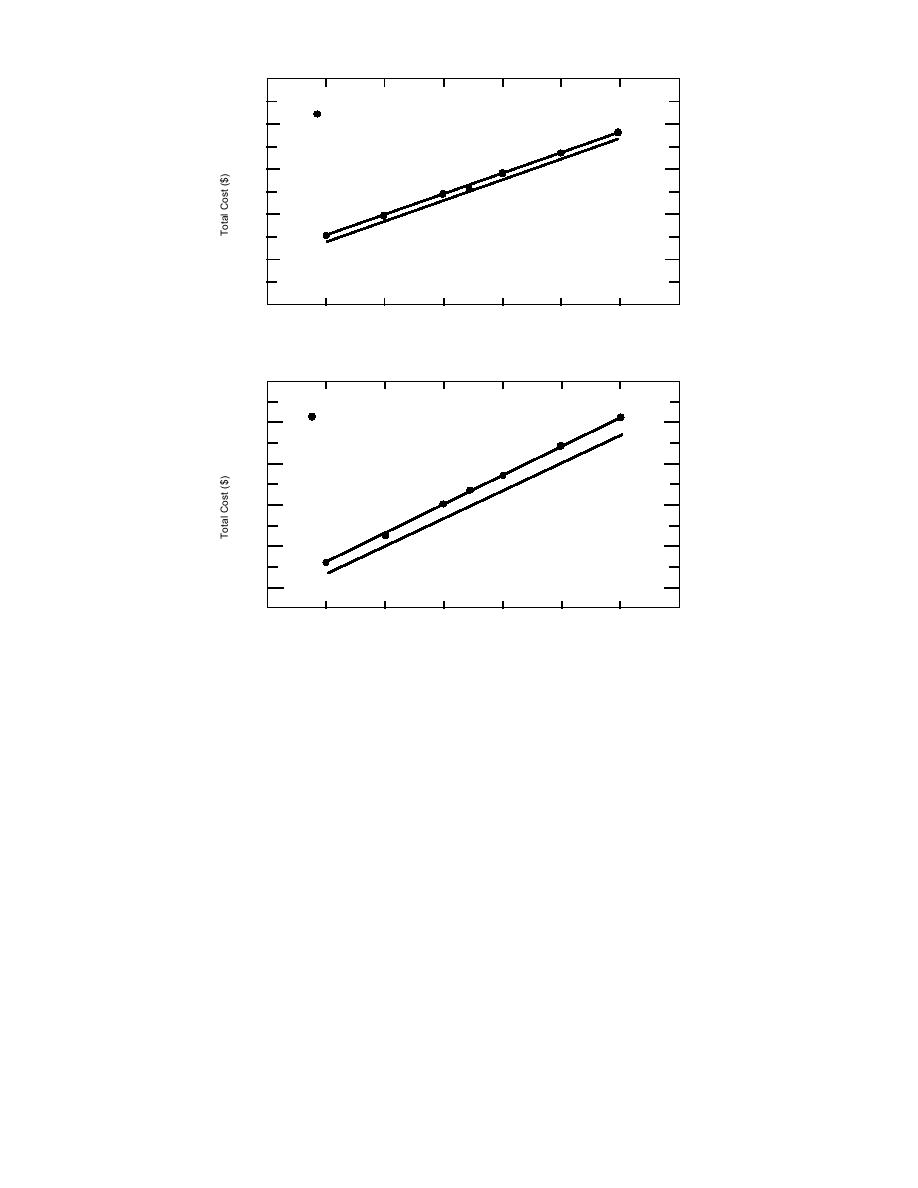
a. April transits.
400 x 103
Modeled Results
380
360
Linear
Fit
Eq. 5
340
320
300
20 x 10 3
17
18
19
13
14
15
16
Cargo Ship Rate ($/day)
b. August transits.
Figure 13. The effect of cargo ship rates on total shipping costs.
D show that the simple equation insignificantly
For this scenario, eq 5 then becomes:
underpredicts the numerical model.
TCApr = (,450 23.588 days) + (IBR 22 days)
For August transits, the linear fit to the numeri-
cally modeled results is
and
TCAug = 3.310 IBR + 3,166
TCAug = (,450 13.601 days) + (IBR 4 days),
and the corresponding r2 statistic is 0.9775. The
and the results of varying IBR are presented in
change in total cost is 3.31 times the change in the
Table 18 and Figure 14. The least-squares linear fit
icebreaker rate. The difference between the simple
to the modeled results for April was
prediction equation and the numerical result is
similar in magnitude to the April differences.
TCApr = 21.810 IBR + 6,808
Finally, MF was varied while holding CSR and
IBR constant. CSR was held at ,450/day while
with an r2 statistic of 0.9995. The slope shows that
IBR was held at zero. For this scenario, eq 5 then
becomes
for every
||content||
change in the icebreaker 's daily rate,
there is a resulting .81 change in the total cost
TCApr = (,450 23.588 days) + MF
of transit. Again, the difference values in column
39


 Previous Page
