50
16
45
14
40
12
35
10
30
γ (h)
γ (h)
25
8
20
6
15
4
10
2
5
0
0
27
0
3
6
9
12
15
18
21
24
0
3
6
9
12
15
18
21
24
27
h
h
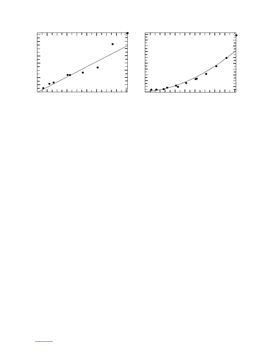
a. 21 June 1992.
b. 19 December 1991.
Figure 19. Typical variogram plots of FERF data sets.
APPLICATIONS
mine pavement stiffness and deflection. Using the
Variogram analysis allows one to quantify the spatial
knowledge of the lengths over which any particular
variability of the thaw depth for various types of ter-
indicator value is correlated can translate into substan-
rain. Standard statistics (i.e., standard deviation, histo-
tial savings by optimizing pavement evaluation tests.
gram) do not relate to the relative positions of the test
Temporal and spatial variability on soil strength has
data but are essential information on the variation of
been investigated for off-road mobility to define the
thaw depth. The correlation range and variation of thaw
soil strength uncertainties, and for forecasting soil
depth over a terrain can be used to quantify the thaw
strength (Mason et al. 1997). Mason et al. used soil
depth variability in models where thaw depth is needed,
strength data to develop coefficients to forecast the
such as mobility performance models.
changes of soil strength with time, and spatial relation-
The depth of thaw causes a significant impact on
ship on soil strength with the terrain elevation using
vehicle mobility (Shoop 1990). Soils with a thawed
variogram and kriging methods.
layer can be saturated due to snowmelt, rain, and water
drawn to the soil during the freezing process. The under-
DISCUSSION
lying frozen layer traps this moisture, so the upper soil
layer is wet and weak. A thaw-depth algorithm has been
The average thaw depth versus the standard devia-
incorporated into a vehicle performance model called
tion of all the data sets from all sites is shown in Figure
NATO Reference Mobility Model II (NRMMII) (Rich-
20. The variance in the thaw is proportional to the thaw
mond et al. 1995). NRMMII predicts maximum attain-
depth according to eq 7 and 8.
able speed of a vehicle operating on a terrain (Ahlvin and
σthaw = 0.3007 mthaw
Haley 1992). The terrain is divided into a terrain unit
(7)
for corresponding soil type, soil strength, soil wetness
σthaw = 0.1513 mthaw
index, soil strength, obstacles, and surface roughness.
(8)
Thaw depth is an input variable to a terrain or scenario
where σthaw is the standard deviation of the thaw depth
file for NRMMII and is assumed uniform throughout
the terrain or can be specified for each terrain unit.
and mthaw is the average thaw depth (cm). The controlled
Kestler (1996) used statistical, geostatical (vario-
test section in the FERF has a slightly smaller slope.
gram), and regression analyses to establish whether
At sites where data was collected with thaw pro-
variation in subgrade reflects the performance of a test
gression (i.e., Alaska), spatial correlation ranges are
section. Her study concluded that thaw depth, water
fairly constant as the thaw depth progresses. In Swan
content, percentage of water standing, and soil strength
Lake, Minnesota, data was collected with time but no
influenced the test section performance. Also, Kestler
correlation range was found as discussed previously.
et al. (1994) identified spatial correlation as a function
The data sets were collected at various sampling
of distance using the falling weight deflectometer
scales. For example, at Swan Lake, the data were mea-
(FWD) data to assess the overall pavement structure.
sured within the confines of the shallow depression,
and in the case of the FERF, it is the dimension of the
The FWD is towed by a vehicle and is used to deter-
16
to contents


 Previous Page
