modeled. The specimen was initially at 1C, then the
by the surface effects of the solid:
top temperature was gradually ramped down to 0.5C.
L = LB LΨ
The thermal conductivity of the specimen was com-
(74)
puted as a geometric mean of the thermal conductivi-
where L is the chemical potential of the liquid in the
ties of soil solids, ice, and water during freezing. Fig-
film, LB is the chemical potential of the bulk liquid,
ures 9a and b show typical results. The model predicts
and LΨ is the depression in the chemical potential from
behavior of the soil column during freezing and the
values are reasonable.
bulk water caused by the presence of the solid surface.
Black and Miller (1985) applied a simplified ver-
Gilpin assumed that it had the form of a power law
sion of the rigid ice model to laboratory test results on
relationship:
a silt. They assumed that the liquid water content and
LΨ= ayα
(75)
the unsaturated hydraulic conductivities were simple
Brooks-and-Corey-type exponential functions of φ (e.g.,
where y is the distance from the soil particle surface
and a and α could be adjusted as needed.
Brooks and Corey 1964). Heave and frost penetration
rates and temperature gradients in the unfrozen soil were
The chemical potential of the bulk water is given
input variables, while temperature gradients in the fro-
by (an integrated form of eq 19)
zen soil and heaving pressure were outputs. The model
LB = Lo + VL (PL - Po ) - SL (TL - To )
accurately predicted temperature gradients, but predict-
(76)
ed heaving pressures to be about half of those mea-
where Lo is the chemical potential at a reference con-
sured, indicating problems with the experimental pro-
cedure that were later found to exist.* The rigid ice
dition, (Po, To). Substituting eq 75 into eq 74 and 74
model is now available in the form of a MathCad 5.0+
computer program (Black 1995).
that the temperatures of the bulk and film water are
The rigid ice model has now been developed into an
equal leads to the following expression for the varia-
engineering tool for prediction of heaving due to one-
tion of pressure in film water, with a distance from the
dimensional heat loss. Using the rigid ice model as a
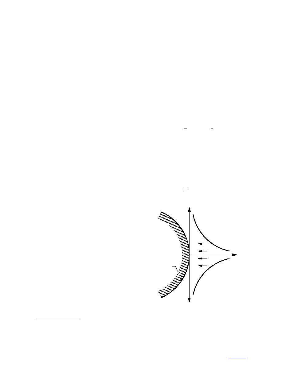
solid surface (Fig. 10):
basis, Sheng (1994) developed a numerical model of
a
frost heave. This model, called PC-Heave, predicts
(PL - Po ) = y -α .
(77)
heave for stratified soils and unsaturated layers. Input
VL
variables for PC-Heave are the number of soil layers
and their thicknesses, the dry densities, water contents,
P
thermal and hydraulic conductivities and percentage
saturation of the soil layers, the boundary temperatures
at the top and the bottom, the depth of the groundwater
Bulk Water
table, and one unfrozen water content at a subfreezing
PL
temperature per FSL (a calibration factor). The model
predicts heave, location of ice lenses, frost penetration,
segregation temperature, and suction in the pore water
of the frozen fringe with time.
g
The modeling equations are the mass and heat bal-
y
ances at the base of the warmest ice lens and for the
frozen fringe, Darcy's Law, and the expression for the
Surface
pore water pressure in the frozen fringe that incorpo-
rates the generalized Clapeyron equation (Sheng 1994).
The model has been verified using both field and labo-
L
ratory soil freezing information.
Gilpin
Gilpin (1979, 1980) developed a model very similar
L
to the rigid ice model. He assumed that the chemical
potential of the water in the adsorbed film is lowered
Figure 10. Gradient in film water pressure next
to a soil particle as described by Gilpin (1980);
note similarity to ion distribution according to
* Personal communication, Dr. Patrick Black, CRREL, Hanover, New
the diffuse double layer theory.
Hampshire, 1999.
15


 Previous Page
