type I (Gumbel), II (Frechet), or III (reverse
Weibull) extreme value distribution. How-
ever, for dealing with ice load extremes, the
peaks-over-threshold (POT) approach is bet-
ter for the following reasons:
At a given location freezing-rain
storms occur infrequently and some
winters will have no measurable freez-
ing rain. In those years the maximum
ice load is zero, which would have to
be considered part of the extreme pop-
ulation in the epochal method.
In other years there will be more than
one severe ice storm, each of which
may cause larger ice loads than the
most severe storms in milder years.
The epochal method would not in-
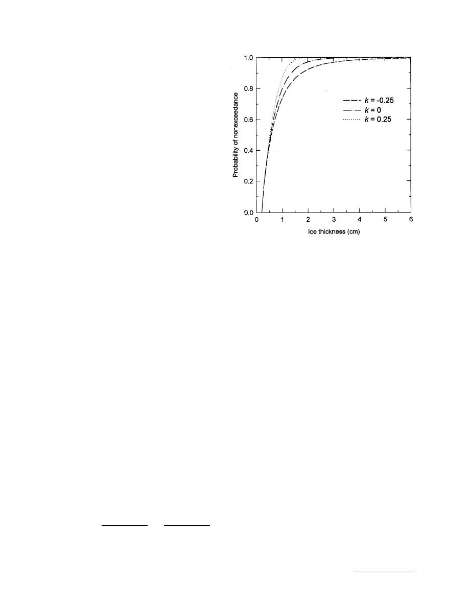
Figure 23. Generalized Pareto distribution.
clude these severe but not-worst-that-
year storms in the estimation of the
parameters of the extreme value distribution.
Because the calendar year ends in the middle of the freezing rain season one could argue
that it makes more sense to choose maximum ice loads for seasons rather than for calendar
years. In a study in which both were tried, the parameters of the extreme value distribution
depended on whether the calendar or seasonal year was used (Laflamme 1993).
These problems are avoided using the POT method because loads are chosen as members of the
extreme population if they exceed a specified threshold load. The excess of the load over this
threshold is used to determine the two parameters of the generalized Pareto distribution (GPD):
kπ0
F(x) = P(X xΩx ≥ u)= 1[1 k(x u)/a]1/k
(4)
= 1 exp[ (x u)/a]
k = 0.
The threshold load is u, the shape parameter is k, and a is the scale parameter. The cases
k = 0, k < 0, and k > 0 correspond to the extreme value distribution types I (shortest infinite tail),
II (infinite tail length), and III (finite tail length, x < a/k) shown in Fig. 23. Typically k ranges be-
tween 0.5 and 0.5. If the data are correctly described by a GPD, then k is not dependent on the
load chosen as the threshold, as long as the threshold is chosen high enough.
Probability weighted moments (Abild et al. 1992, Wang 1991, Hoskings and Wallis 1987) are
often used to determine the distribution parameters k and a. This method is particularly efficient
for distributions with k < 0, which seems to be generally true of extreme ice load data. Estimates
of the GPD parameters are provided by
4b1 - 3bo + u
4b - 3bo + u
k=
k= 1
bo - 2b1
bo - 2b1
a = (bo - u)(1 + k) a = (bo - u)(1 + k)
39
Back to contents page


 Previous Page
