j
j
*j
Rm,n ( f ) = Xm ( f ) * Xn ( f ) ,
are overlapped by an integer number of points.
(21)
The Fourier transform of the jth block from chan-
nel m will be
where m and n are sensor indices. The final esti-
mate of the spatial correlation matrix is formed by
1 L1
∑ alxm (l + j nshft)e i2πf(l∆t)
averaging over the block index,
^j
j
=
Xm ( f )
L
(20)
l=0
nblks
1
∑ Rm,n
j
Rm,n ( f ) =
.
(22)
where the al are time-domain window taper
nblks
weights. The window tapers decrease the bias in
j=1
the estimate by ensuring that the ends of each
The formation of the cross-power function be-
segment of data are gradually tapered to zero.
tween two vectors produces a vector that has a
A variety of window taper functions may be
phase angle that is the difference in phase between
applied, each having a different impact on the
the two constituent vectors. For waveforms pro-
properties of the resulting spectral estimate. Har-
duced by a stationary source and recorded by chan-
ris (1978) presents an excellent overview on win-
nel m, the Fourier transform at any given fre-
dow tapering strategies for harmonic analysis
quency will be a randomly oriented vector. Thus,
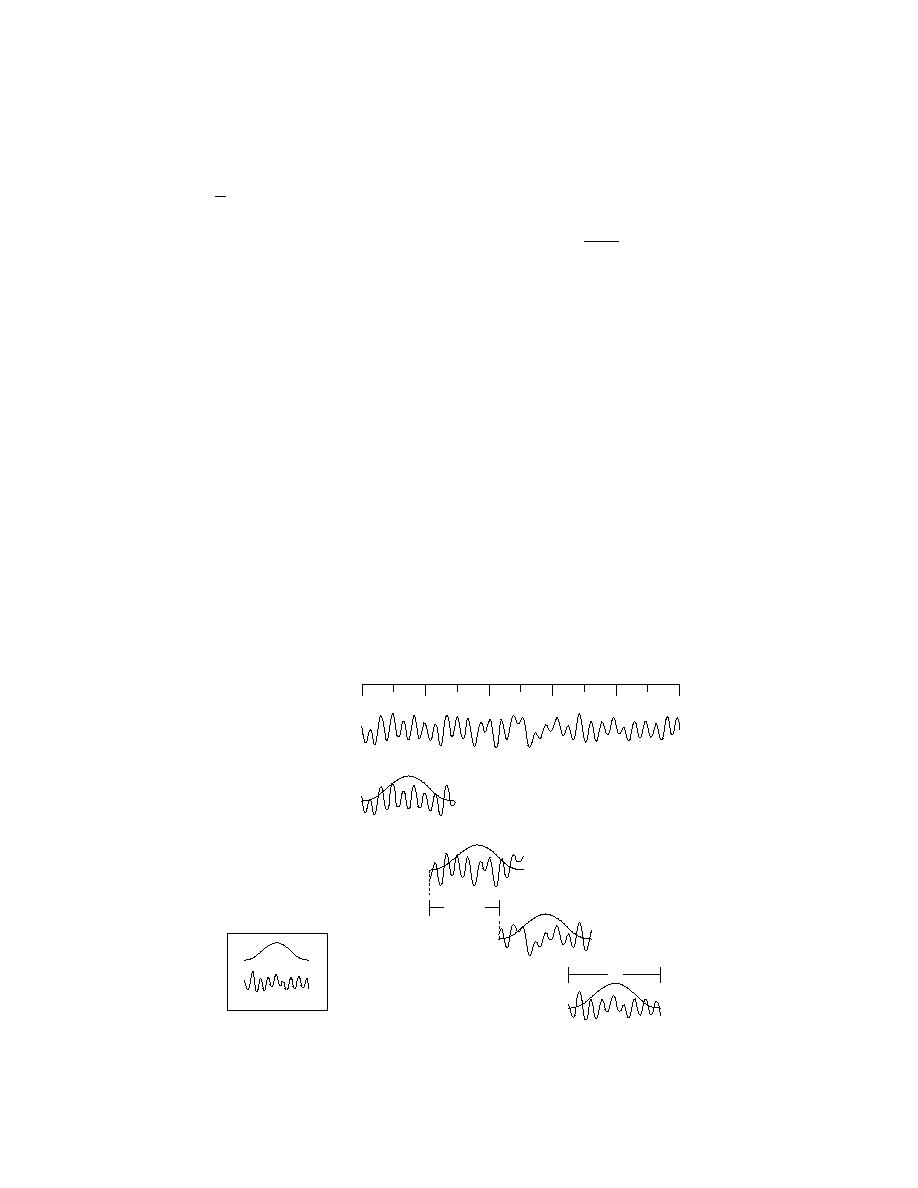
problems. Figure 3 graphically illustrates the
the OBAFFT gives, for each block of data in chan-
overlapped (OBAFFT) segmentation.
nel m, a series of vectors with random phase angles.
In an array of sensors recording real data, the quan-
2.3.2. Formation of spatial correlation matrix
tity to be measured is the phase difference between
The cross-power function between all pairs of
channels. The final estimate of the spatial correla-
sensors in the array is calculated for each block of
tion matrix given by eq 22 is therefore an average
data in the OBAFFT method. The final estimate of
of several phase angle difference matrices, which
the spatial correlation matrix is formed by averag-
becomes less variable as the number of blocks
ing over the block cross-power matrices.
increases. This assumes that the phase difference
Using eq 20, elements of the cross-power matrix
between channels is not changing with time.
for the jth block are
Time (s)
0
0.2
0.4
0.6
0.8
1.0
Xm
nblk 1
nblk 2
nshift
nblk 3
Taper
L
Data
nblk 4
Figure 3. Segmentation and overlapping of a time-domain component of the
signal vector. Each tapered block is transformed into the frequency domain via
an FFT.
6


 Previous Page
