tion, the estimation and conditioning procedures
erate the cross-power matrix in the beamforming
of the spatial correlation matrix are given.
equations. A confidence interval for the variance
in the cross-power matrix is developed. This is
followed by a discussion of the experimental set-
2.1 Beam-power response function
Assme an array of M sensors have vector loca-
u
ting, data acquisition procedure, and seismic ar-
tions R m in the xy plane
ray characteristics. Processing results are then given
for an impulsive acoustic source, a pure seismic
R m = xm +ym
2
2
source, and a moving M60 tank. We obtain accu-
rate wavenumber estimates from the beamformer
for all three source types. Next we show that small
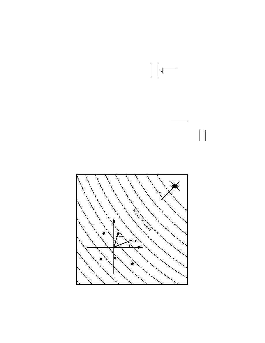
as shown in Figure 2. Each sensor is a spatial
variations in the parameters used to estimate the
wavefield sample point that records over time.
cross-power matrix contribute to wavenumber
Such a collection of sensor data is termed the signal
bias effects. These bias effects are summarized for
vector. A wavefield containing a single plane wave
a variety of block lengths, block overlaps, and
source sampled at locations R m may be repre-
window types.
sented by a signal vector with components:
R m u ko
xm (t) = s t +
+ nm (t) ,
(1)
2. BEAMFORMING PRINCIPLES
c
The discussion given here follows Capon (1969)
where k o is the wavenumber k o = 2πf /c , u ko
and Johnson (1982). First, a general expression for
an FK beamformer power function is given. The
is the unit vector direction of the source, nm is the
standard Bartlett (BT) and high-resolution Capon
background noise field, and c is the scalar wave
maximum-likelihood (ML) beamformer equations
propagation velocity. In the frequency domain,
are obtained. Following the beamformer deriva-
eq 1 is
Source
k0
x
m
Rm
k
θ
y
r
at vector positions r m . The pseudo-plane wave sourre has a
c
R
wavenumber vector k o . The observation wavenumber is k . Dots
() are sensor locations.
3


 Previous Page
