as obtained from the correlation map. The affine parameter
Magnitude (kms)
30
estimation chosen is a least-squares fit to the locally trans-
RMSEcomplete = 0.88498
lated patch. The Peak Signal to Noise Ratio (PSNR) values,
RMSEgood = 0.13614
d
= 0.98145
25
complete
calculated using Eq. 4, are provided in Table 1.
d
= 0.99318
good
n
= 2650
complete
n
= 1930
good
n
= 548
20
255
deformation
]
P SN R = 20 ∗ log10[
(4)
σ|Image1-Image2|
15
where σ is the standard deviation, I mage1 and I mage2 is
10
the image pair under consideration. From the table it is ev-
ident that the PSNR value between I mage2 and the mo-
5
tion compensated images increases with increasing motion
0
model complexity.
0
5
10
15
20
25
30
ISW Vectors
5. Conclusion
Direction (degs)
280
RMSEcomplete = 7.7171
RMSEgood = 1.268
Localizing and parameterizing discontinuities is an im-
260
dcomplete = 0.97229
d
= 0.98891
good
portant landmark for sea-ice research. Due to the low tem-
240
ncomplete = 2650
ngood = 1930
poral resolution of the SAR images, this type of information
220
n
= 548
deformation
is paramount input into numerical models for interpretation
200
of events between SAR scenes. This paper describes a hi-
180
erarchical method to estimate the parameters of a discon-
160
tinuous motion field such as the ones captured by the ERS-
140
1 SAR imagery in three stages. The hypothesis of using
120
a finer sieve to filter out coarse motion models iteratively
100
seems to be validated with the observed improvement in the
80
PSNR values of the motion compensated images.
80
100
120
140
160
180
200
220
240
260
280
The comparative results between the estimated vectors
ISW Vectors
and the ISW ground truth vectors indicate that hierarchical
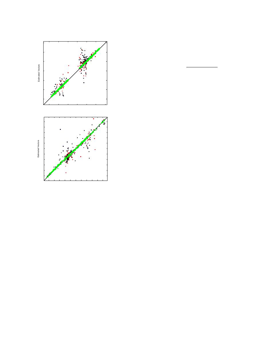
Figure 5. Scatter plot of the estimated vec-
phase correlation is ideal for the estimation of the global
tors v/s ISW vectors for the entire sequence of
motion. This is mainly due to the inherent robustness of
images during ISW. Green indicate the good
phase correlation to illumination variation and its ability
points, blue are the deforming points and red
to capture large translational components without getting
are points we can not explain.
caught in local minima. Additionally, the usage of the Fast
Fourier Transform in the calculation of the phase correlation
term makes the computation significantly faster then optic
flow methods.
The second stage involves isolation of discontinuous re-
to ISW vectors. Including flagged points undergoing de-
formation we can account for 93.5% of all the data points.
gions using local piecewise linear model followed by the
The remaining 6.5% of data are displacement results greater
third stage of estimating affine parameters along regions of
discontinuities. Under the assumption that the net motion
than 400m which we can not account for using a correlation
is actually composed of a large global motion component
map. These points mainly correspond to regions where the
and small local deformations, this method captures the large
gradient of the velocity is high and, in principle, requires
global motion component and the local deformation using
a higher-order motion model to localize the position of the
an affine motion model.
discontinuity accurately. Also indicated in the scatter plot
are the RMSE (Eq. 2) and index of agreement (Eq. 3) for
As a subsequent stage to the current research, the esti-
the complete data set and the "good" data set indicating a
mate of the local deformation could be improved using ro-
high accuracy between the ISW vectors and our estimated
bust parameter estimation techniques and also inclusion of a
motion vectors.
motion model such as the quadratic. Another possible track
To improve upon the estimated parameters, an affine mo-
for future research would be a feature-based approach in
tion is imposed onto the local piece-wise linear motion.
tandem with global motion estimation in order to improve
This is performed specifically in the regions of discontinuity
the overall robustness of the estimated global motion.


 Previous Page
