original test site on Second Avenue in
20
Berlin. The pipe is 20.3-cm (8-in.) I.D.
ductile iron set 1.5 m (5 ft) deep. Mate-
16
rial 6 is the pipe and water, material 4
represents the backfill area around the
12
pipe, material 7 is the extruded poly-
styrene insulation boards, and materi-
8
als 2 and 11 are the surrounding earth
and ledge material, respectively. The
4
specific dimensions and materials asso-
ciated with each zone might change, de-
0
Jan Feb Mar Apr May Jun Jul Aug Sep Oct Nov Dec
pending upon what the designer wishes
to experiment with. For instance, in our
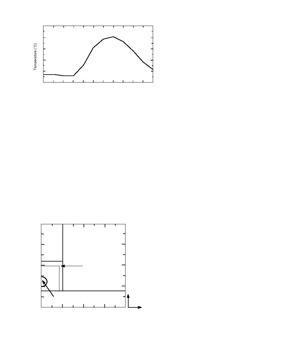
Figure 3. Berlin, New Hampshire, filter plant water temperatures.
modeling we varied the pipe depth, in-
sulation board thickness, and the width of the top
data, which we will show later, indicates that
insulation board to see the effect these changes
early in this year the water at the filter plant was
would have upon the temperature profiles.
colder than the ground for portions of the year.
We thought that the pipe on Second Avenue
Figure 3 shows the water temperatures we used
could be installed about 1.5 m (5 ft) deep, but
in our simulation.
ledge was possible anywhere from 1.4 m to 2 m
In our numerical simulations we model to a
(4.5 ft to 6.5 ft). In Figure 4, material 11 was ledge
depth of 10 m (32.8 ft), which can reasonably be
and material 2 was a "silty sand" commonly found
assumed to represent the depth of zero annual
in the area. The backfill material 4 is a sand. As
temperature amplitude (Phukan 1985). This is the
mentioned above, we varied the extruded poly-
depth at which the effect of the changing surface
styrene insulation (material 7) dimensions during
temperature is not noticeable. At this bottom
the modeling process to investigate the effective-
boundary we apply an average value of the geo-
thermal heat flux of 0.063 W/m2 (Lunardini 1981)
ness of different shield thicknesses and place-
ment. Table 1 lists the materials and their prop-
moving upward into the mesh.
erties.
During the numerical simulations, we defined
a failure as the 0C isotherm touching the pipe.
SECOND AVENUE
This is a conservative approach, since water will
remain at 0C for some time before it freezes due
Figure 4 is an example of the basic FE configu-
to its latent heat. For the initial runs we did not
ration used to model what we initially expected
apply any water temperature boundary condi-
the soil and pipe configuration to look like at our
tion to the pipe. This would be similar to a
pipe with no flowing water. Commonly, wa-
0
ter flowing in the pipe brings heat into the
insulation shield, so modeling without wa-
Material 2
Material 4
ter flow is usually a more conservative pro-
0.5
cedure.
The output from a numerical simulation
is presented in graphical form by either
graphs or contour plots. By watching how
1.0
the 0C isotherm progresses with time, the
Material 7
effectiveness of the insulation shield can be
determined. Figure 5 shows a time series pro-
gression of five isotherms around and into
1.5
a shield. Notice how the isotherms wrap
around the shield and start to intrude not
y
Material 6
Material 11
only at the top but also at the lower right
x
corner. This is due to the higher-conductiv-
2.0
0
0.5
1.0
1.5
2.0
ity ledge at the bottom of the shield. This
contour type of output is extremely helpful
Figure 4. Physical layout of FE-modeled domain.
4


 Previous Page
