tical line of symmetry through the insulation and
month were used as our surface temperatures in
pipe. This mesh consists of a series of triangular
the model.
elements arranged in zones that accurately repre-
Actual surface temperature is usually different
sent the physical configuration of the material
from air temperature and can be determined by
being studied. The density of the element spacing
the use of so-called "n-factors." These factors re-
depends upon the temperature gradients expected
late the effect that surface material has upon the
in any zone. Areas of steep gradients (high tem-
surface temperature (Lunardini 1981). By multi-
perature change) should have elements that are
plying the air temperature by the appropriate
spaced closely together. Thus, in Figure 1 there
material n-factor, the surface temperature can be
are areas that have very closely spaced elements
determined. A good illustration of the surface tem-
representing the insulation boards. These are the
perature difference is the hot temperatures found
darker vertical and horizontal bands evident in
in summer on a black asphalt surface, which will
the figure. The insulation boards are placed in an
normally be several degrees hotter than the air
inverted U immediately around the pipe, which
temperature.
is the darker half-round object at the lefthand
Using air temperature as our mesh surface
side of the mesh. The dark bands extend beyond
boundary temperature gives us, on average, a
the boundaries of the insulation boards because it
somewhat colder surface than the actual would
is easier to generate them as a continuous band
be. This was desirable from a conservative point
throughout the mesh and then just designate the
of view so our shield design would be somewhat
board itself in the material file by their coordi-
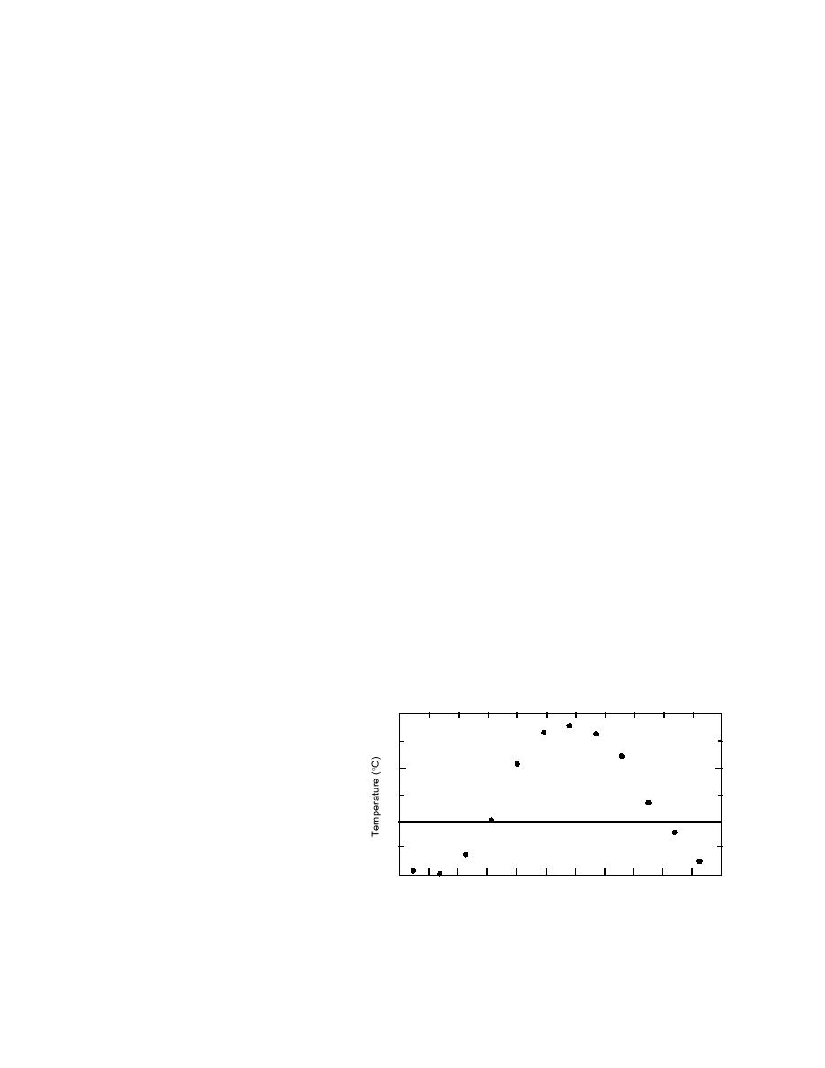
overdesigned. Figure 2 is a graph of the air tem-
nates. For example, the top horizontal board ex-
peratures determined from our records. The time
tends from the lefthand side of the mesh to the
scale is in months and represents a full year start-
righthand edge of the vertical band. The vertical
ing in January.
board extends from the bottom of the horizontal
Water temperature was more difficult to deter-
band to just below the bottom of the pipe. Each of
mine. We obtained monthly treatment and filter
the other materials present in the physical con-
plant outflow water temperatures for 1992 and
figuration is designated by the appropriate coor-
part of 1993 and used these records to estimate
dinates of the zone of elements in the mesh. The
the water temperature in the pipe. There can be a
program uses this information, along with the
significant error in these temperatures because
thermal conductivity, density, specific heat, la-
the water temperature will change as it travels
tent heat, and phase-change temperature of the
throughout the distribution system. How it
components to determine heat transfer through-
changes is not known. For instance, in the winter,
out the region under study. More information on
the water from the plants might cool significantly
finite element (FE) modeling can be found in text-
as it travels through pipes that are buried in
books on the subject (Segerlind 1984).
ground that is below freezing. Conversely, since
Once the physical configuration is determined,
a large portion of Berlin's water is from a surface
all the boundary conditions that will affect the
source, it may in fact be cooler than the ground
mesh temperatures have to be determined for a
for a large part of the season. The preliminary
full year's cycle. In our case, the surface
temperature, water temperature, and
20
geothermal heat flux (heat generated
within the core of the earth that slowly
filters up to the surface) were the bound-
10
ary conditions that were needed for our
problem. Along the vertical line of sym-
metry, the boundary condition is adia-
batic (zero heat flux).
0
The surface temperatures used in the
model were determined from monthly
extreme air temperature records for the
10
Berlin area from 1926 to 1992. From the
Jan Feb Mar Apr May Jun Jul Aug Sep Oct Nov Dec
records, 1972 appeared to be the cold-
Figure 2. Average air temperatures from 1972 used to represent
est year, and the average of the coldest
FE surface temperature.
and warmest temperatures within each
3


 Previous Page
