The amount of scatter, relative to the least square fit, increases in the flux range from
approximately 50 to 400 W/m2. Some of this scatter is no doubt due to the comparison of
the average flux conditions with calculated fluxes based on the instantaneous observation
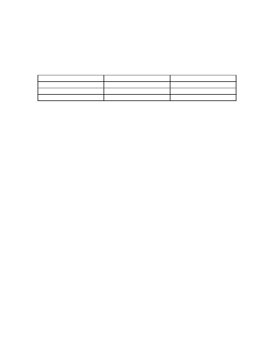
of cloud amount on the hour. Table 2.6.1 presents the equation for the least square fit and
its correlation coefficient for the total solar flux and each of the flux components.
Table 2.6.1 Equation of fit (forced through the origin) and correlation coefficient for Grayling I.
R2
Solar Flux
Equation of Fit
Total
y=1.0361x
0.8049
Direct
y=1.1353x
0.8631
Diffuse
y=0.8757x
0.3752
The comparison of the diffuse components shows considerable amount of scatter as
evident by the low correlation coefficient. There are a number of data points where the
calculated is on the order of 100 to 200 W/m2 greater than the measured value. This
relatively large difference is due in part to inappropriate cloud representation. This
includes both the cloud amounts and the implicit cloud optical depth as discussed earlier.
Figure 2.5 explores the impact of cloud conditions on the difference of the calculated
total solar flux minus the total solar measured flux. Some interesting features are
observed in Figure 2.5. The range of flux differences is smallest when there is no low
cloud (clear, middle, high, or middle plus high). When there are only low clouds the
differences are evenly distributed from 300 to +300 W/m2. When there are low clouds
plus another cloud type (low + middle, low + high, or low + middle + high), the
calculated flux tends to be greater than the measured flux. The cloud optical depth is a
function of the cloud thickness. The cloud model does not directly use cloud optical
depth or cloud thickness. One of the reasons for this is that cloud thickness and cloud
optical depth are not reported meteorological variables.
10


 Previous Page
