

100
2000
Water Level (m)
1600
80
60
1200
Q (m3)
800
40
Pool Depth (m)
20
400
0
0
7
0
1
2
3
4
5
6
X = D100.5
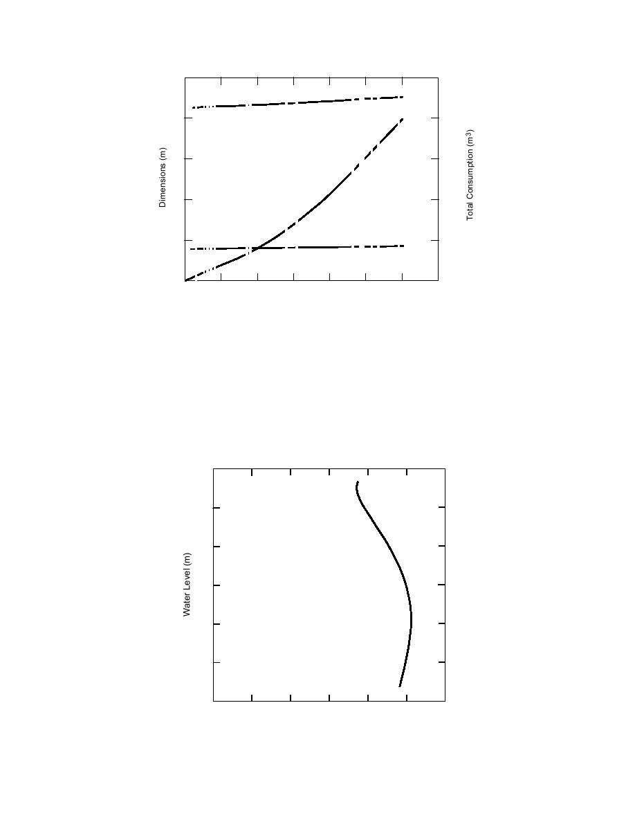
Figure A5. Period 3 (consumption) dimensions and water consumption, and
polynomial curves fitted to data.
over the period is less than 0.1, so we may treat H as a constant for the period, H =
15.5 m. In addition, solution of eq A7 requires an integration constant. If we as-
sume that changes in well radius become small near the end of the period (i.e., the
well dimensions stabilize) we may solve eq A7 with dR/dx = 0 to obtain an integra-
tion constant, R(6 m) = 11.9 m.
Figure A6 shows the resulting prediction for the R(L) obtained by solving eq A7
85
86
87
88
89
90
91
7
8
9
10
11
12
13
Radius (m)
Figure A6. Predicted period 3 cavity shape, from eq A7.
30

 Previous Page
