solved for each set of values in Table A1. Instead, we generated polynomial curves
that give very good fits to the data and reduce the influence of uncertainties in
these measurements.
There are three periods of interest:
1. From initial startup on 12/8/92 to the fire-induced shutdown on 3/1/94,
2. From restart on 12/2/94 to the start of consumption on 1/30/95, and
3. The period of consumption ending 12/29/95 after our six collector deploy-
ments.
Periods 1 and 2
For the first two periods, no consumption occurred. Setting dQ = 0 and using the
substitution x = D 60, eq A7 becomes
dR
= c( x)R( x) ,
(A9)
γ p dL
dH
dx
π 1 γ dx α dx
.
p
where
c( x) =
2αH( x)
The solution of eq A9 is simply
x
∫
R( x) = R0 exp c( x)dx ,
(A10)
0
where R0 = R(0).
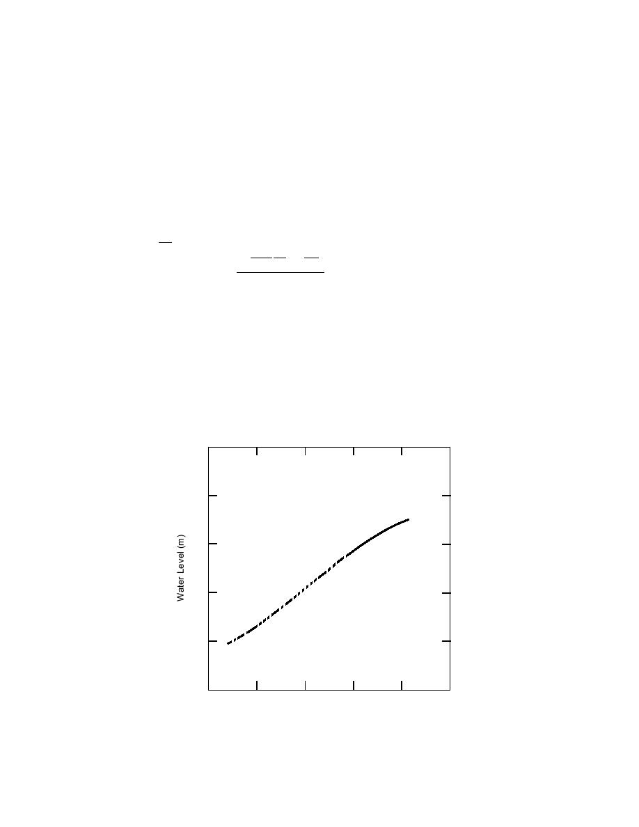
Figure A3 shows the measured water levels and a third-degree polynomial ap-
proximation for L(x) over period 1. Note that H(x) = x + 60 L(x). Figure A4 shows
the resulting solution for α = 2π/3 and R0 = 15 cm (the radius of the hot-water drill)
plotted as R(L). This curve represents the predicted shape of the well cavity formed
100
90
80
70
60
50
0
10
20
30
40
50
X = D60 (m)
Figure A3. Period 1 (prefire) water level vs. depth and third-degree
polynomial curve fitted to data.
28


 Previous Page
