40
Ellipsoidal Pool Shape
R(0) = 0.15 m
50
60
70
80
90
0
10
20
30
40
50
Radius, R(L) (m)
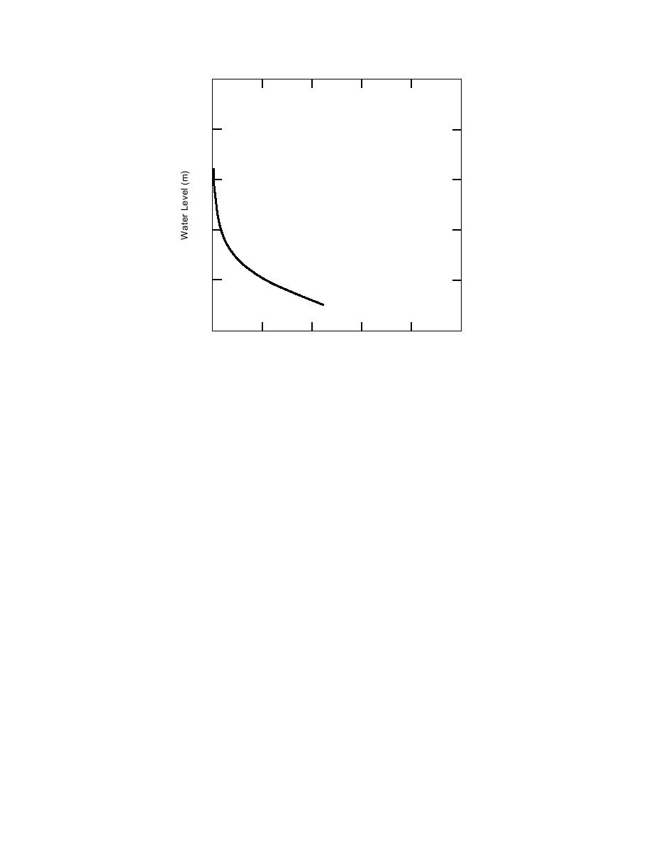
Figure A4. Predicted period 1 cavity shape, from eq A10.
during period 1. There are two main problems with these results. First, the pre-
dicted radius at the level of the freeze-back ice cover, R(82.6 m) = 16 m, is substan-
tially larger than that estimated from down-hole video images (8 2 m). Second,
the observed cavity appeared to flare out at its upper end and become more verti-
cal toward its bottom; that is, it appeared to be bell-shaped. The predicted shape
actually has the opposite trend: it is narrow (with near vertical walls) at its upper
end, and it flares out towards the bottom.
The most likely cause for the poor prediction by eq A10 is that it does not ac-
count for water percolation out of the well (dQ ≠ 0 in eq A7). Based on other
Rodriguez wells, Lunardini and Rand (1995) assumed that percolation would cease
at an ice specific gravity greater than 0.72, corresponding to depths below 74 m.
This generally agrees with Williams (1974), who expected that percolation from the
first South Pole Rodriguez well would cease at about 76 m. Modeling the percola-
tion from the well is beyond the present scope of work and would introduce its
own uncertainties. A more satisfactory approach would be to measure the cavity
radius as a function of depth using a device lowered into the well.
Period 2 covers the two-month period after restarting the well on 12/2/94 but
before consumption began on 1/30/95. The well had frozen back about 11 m dur-
ing the nine-month shut down after the fire. Although percolation would not be
significant during period 2, new ice had not been melted before the start of con-
sumption. That is, there is no need to analyze period 2 to determine the volume of
ice melted that released micrometeorites into the well.
Period 3
During the period of water consumption, the water level was below 85 m, and
we would expect percolation to be zero. Thus, eq A7 may be used to relate changes
in well dimensions to the rate of water consumed. Figure A5 shows the polynomial
curves fitted to L, H, and Q data for period 3 (with x = D 100.5). Note that dH/dx
29


 Previous Page
