peratures from the same time period were
35
Surface (94-95)
used as our pipe temperatures.
FE Regression
Figures 19 and 20 also show the results
25
Regression of Actual
Surface Temperature
from our numerical model. In Figure 19, the
numerical model overpredicts the inside
15
shield temperatures from September until
about the first of December, but it does very
5
well until the end of data in March. The
overprediction is in part because our nu-
5
merical pipe temperatures (from the treat-
ment plant) are warmer than the actual pipe
15
temperatures during September to Decem-
ber. The outside-the-shield numerical tem-
25
peratures are at first warmer than the ac-
3 Sep 3 Oct 2 Nov 2 Dec 1 Jan 31 Jan 2 Mar 1 Apr
tual, until about mid-November. From this
1994
1995
point until the end of December they repre-
Figure 21. FE surface temperature vs. actual surface tem-
sent the actual temperatures well. From then
peratures, Laboissiere Street.
until the end of data in March our numeri-
cal model is somewhat colder than the ac-
tual temperatures.
15
The numerical model did poorly on pre-
Actual Surface
dicting the overall frost penetration as com-
FE Surface
10
pared with the control string temperatures
in ledge. The maximum frost penetration
5
predicted by our numerical model was
roughly 1.8 m (5.9 ft) in about the mid to
0
end of February. The actual maximum frost
penetration was about 1.1 m (3.5 ft) during
5
the first part of March.
The colder numerical temperatures and
deeper modeled frost penetration could be
10
due to our ledge thermal conductivity and/ r
o
the nature of the regression model and how
15
12 Nov
2 Dec
22 Dec
11 Jan 31 Jan
20 Feb
12 Mar
it represents the actual temperatures.
1994
1995
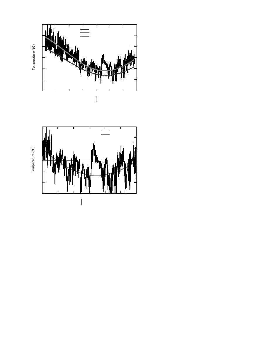
Figure 22 shows a portion of the control
surface temperatures from the beginning of
Figure 22. FE surface vs. actual temperatures.
November until the beginning of March.
Notice that once the regressed surface tem-
perature line goes below 0C it remains there un-
shield design, and the other is one that fits the
actual surface temperature. When the two regres-
til spring. In a normally cold year the actual tem-
sions are compared it shows that the actual sur-
peratures are usually modeled well by this type
face temperature was, on average, over 5.5C
of regression. However, in the winter of 199495,
warmer than the numerical surface temperature.
the actual temperatures rose above this regressed
To better determine how the numerical model
line and above freezing for a significant amount
performed, the top and pipe boundary conditions
of time, as shown in the figure.
were changed to reflect the actual temperatures
To check the effect that the regression line has
more closely. To do this, we need a year's surface
upon frost penetration, we used actual surface
and pipe temperatures covering the model year
temperatures rather than the regressed tempera-
tures as the top boundary condition. The 0C iso-
of interest. We had been gathering data on Sec-
ond Avenue for over a year, and these surface
therm reacted much more realistically in this
temperatures were compared with the available
scenario, with the ground temperatures rising
above 0C during some of the warmer surface
Labossiere temperatures and adjusted to repre-
sent the Labossiere temperatures from March 1994
temperature times. The maximum frost pene-
to March 1995. The treatment plant water tem-
tration time was still around the mid to end of
14


 Previous Page
