

m
=
weight of ice (g)
L
=
length of ice sample (cm)
density of ice 0.9 g/cm3
=
ri
p
=
3.14.
Alternatively, if the ice is melted and the volume of water is measured,
d 2 Vρw
d
t=- +
+
(2)
4 πρi L
2
where V = volume of melted ice (cm3)
rw = density of water 1.0 g/cm3.
Any consistent set of units can be used in the above calculations. In English units the densities of
ice and water are 56 and 62.4 lb/ft3, respectively.
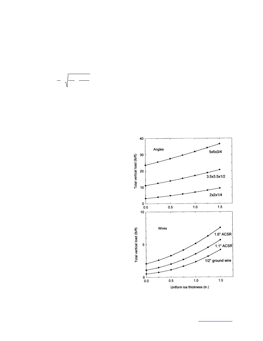
As Eq. 1 and 2 indicate, the equivalent uniform ice thickness represents the ice load. Be-
cause uniformly thick ice forms the most
compact ice accretion, t will always be less
than the maximum thickness of the ice accre-
tion. The actual load, expressed as the weight
of ice per unit length, corresponding to a
specified uniform ice thickness, increases
with the size, or diameter, of the wire or angle
member or branch (Fig. 10). For example, 1-
in. uniform ice thicknesses on 0.5-in. wires,
1.5-in. conductors, and 3.5- 3.5- 1/2-in.
angles weigh 2, 3, and 7 lb/ft, respectively.
In the next section the calculation of ice
loads from hourly weather data using ice
accretion models is discussed. The derivation
of the formula used in the simple model
emphasizes the utility of describing ice loads
from freezing rain in terms of the equivalent
uniform ice thickness.
4. MODELING ICE LOADS
Because ice loads are difficult to measure,
they are often estimated by applying ice
accretion models to weather data. The weath-
er elements that are required for modeling the
accretion of ice in freezing rain are the
present weather code, which indicates wheth-
er freezing rain is occurring, precipitation
Figure 10. Ice loads in pounds per foot corre-
amount, and wind speed. Many models also
sponding to uniform ice thicknesses from 0 to
use air temperature and some use dew-point
1.5 in.
9
Back to contents page

 Previous Page
