Figure 7. Mass flow rate function with and without consumer models, Tr = 55C

1.0

0.8

m/m d

0.6

w/o Consumer Model

0.4

m/m d

0.2

w/Consumer Model

2,000

4,000

6,000

8,000

Time (hr)

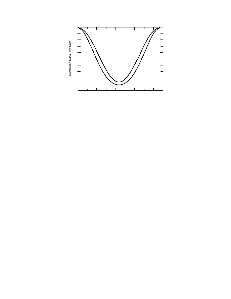
Figure 7. Mass flow rate function with and without consumer

models, Tr = 55C.

have done so in Figure 6. Notice, for the case where the consumer model has been

included, that the maximum value of the normalized mass flow rate is less than

unity. This results from an inconsistency in the design conditions chosen for the

original problem of Chapter 2 and the consumer's radiator model. Our model for the

consumer's radiators assumes design temperatures of 90 and 70C for the supply

and return respectively. With the supply temperature of 120C, the radiator model

will predict a return temperature of 55C, rather than the value of 60C we assumed

earlier. In the case where the return temperature is assumed rather than determined

by a consumer model, the choice of 60C is entirely appropriate, as are the normal

design temperatures of 90 and 70C for supply and return radiator temperatures

respectively. Normal design practice would be to assign these temperatures inde-

pendently. Thus, the lower flow rate that results when we include the effect of the

consumer model illustrates one of the inaccuracies encountered when normal

design practice is followed. If we make the design return temperature for the piping

network equal to that which results from the consumer's radiator model, i.e., 55C,

it results in the normalized mass flow rates shown in Figure 7. From Figure 7 it is

clear that the effect of including the consumer model on the mass flow rate is still

significant once the load condition drops slightly from its maximum value. Aver-

aged over all load conditions, the normalized mass flow rate is 20% less for the case

that includes the consumer model.

To determine what effect this change in normalized mass flow rate will have on

our optimal pipe diameter determined in the example of Chapter 2, we need to

recompute I3, which is the only parameter affected by the changes in the mass flow

rate. We have modified the computer program used in Chapter 2 to calculate I3 by

including eq 3-25 in place of the original normalized mass flow rate as given by eq

2-29. The modified program is included in Appendix B as Program I2-C-GMT. All

constants were assumed to have the same values as before, with A13 taken as unity.

This results in the value of the I3 parameter decreasing by 15% from 44.1 to 37.5 ($

m5.095) because of the effect of the consumer model.

Now we need to determine what other parameters in the solution of the Chapter

2 example would be affected by our consumer model. The only additional effect will

be on the I1 parameter. Since this parameter arises out of heat loss considerations, the

varying return temperature caused by the consumer model will change it some-

what. In the example of Chapter 2, since the supply and return temperature were