(eq 3-17) into eq 3-21, we have
m / m d = (q/qd) (Ts Tr)d/{Ts Ta - (Ts - Ta )-1(Tmg )0 (q / q0 )
} .
2/n1
2
˙ ˙
(3-22)
represents the actual load on the system. The quantity q0 represents the maximum
load for which the consumers' radiators were designed, while the quantity qd
represents the maximum load for which the piping network was designed. These
two "design" loads will in most cases not be equal, as discussed earlier. They will,
however, be related by some "over-design factor," which will be a constant
(q/qd) = A13 (q/q0)
(3-23)
where A13 is the over-design factor for the consumer's radiators (dimensionless).
In the example of Chapter 2, we assumed a sinusoidal form for the variation of the
load over the yearly cycle. In general terms this can be written as
q/qd = A14 + [A15 cos(2πt/8760)]
(3-24)
where A14 is the midpoint of the load curve (dimensionless) and A15 is the amplitude
of the load curve (dimensionless). The midpoint of the load curve A14 is simply the
average of the maximum and minimum loads. The amplitude of the load curve A15
is the maximum load minus the minimum load divided by two.
Now if we combine eq 3-223-24, we have the following expression for the
normalized mass flow rate over the yearly cycle
(Ts - Tr )d (A14 + A15 cos(2πt / 8760))
m / md =
.
˙ ˙
2/n1
(
)
Ts - Ta - (Ts - Ta )-1(Tmg )0 [A14 + A15 cos(2πt / 8760)]/ A13
2
(3-25)
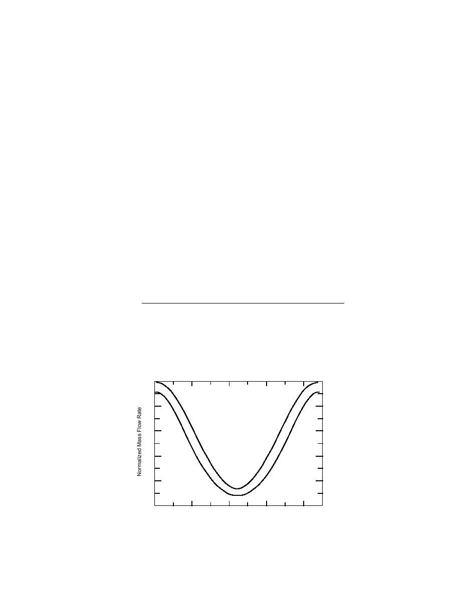
If we select the same values for A14 and A15 as we used in the Chapter 2 example
(0.575 and 0.425 respectively), we can compare the resulting mass flow rate function
of eq 3-25 to the mass flow rate function without the consumer model (eq 2-28). We
1.0
0.8
m/m d
0.6
w/o Consumer Model
0.4
0.2
m/m d
w/Consumer Model
0
2,000
4,000
6,000
8,000
Time (hr)
Figure 6. Mass flow rate function with and without consumer
models, Tr = 60C.
28


 Previous Page
